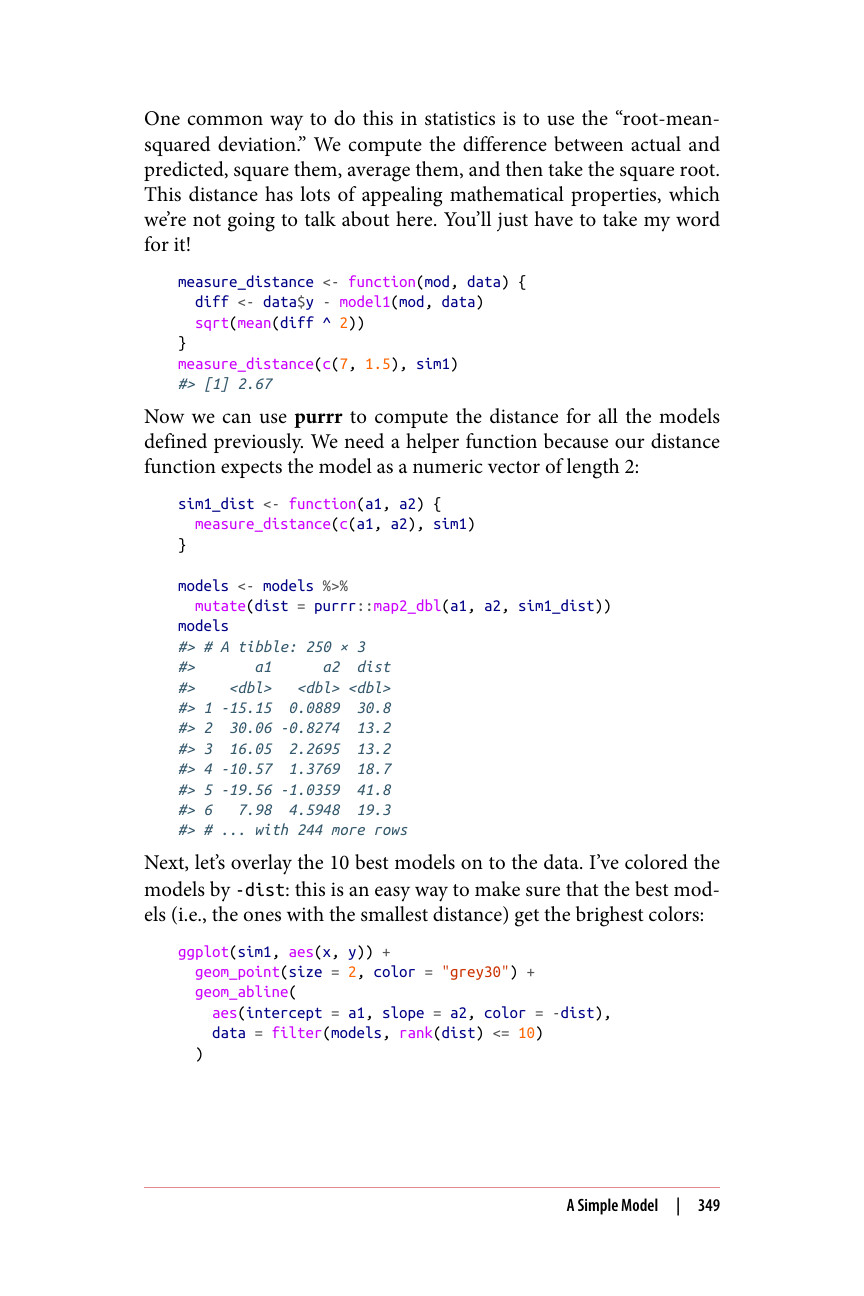
统计学中一种常用的方法是使用“均方根偏差”。我们计算实际值与预测值之间的差值，将其平方，求平均值，然后取平方根。这种距离度量具有许多吸引人的数学性质，我们在这里不打算讨论。你只能姑且相信我的话！

measure_distance <- function(mod, data) { diff <- data$y - model1(mod, data) sqrt(mean(diff ^ 2)) } measure_distance(c(7, 1.5), sim1) #> [1] 2.67

现在我们可以使用 purrr 来计算前面定义的所有模型的距离。我们需要一个辅助函数，因为我们的距离函数要求模型是一个长度为 2 的数值向量：

sim1_dist <- function(a1, a2) { measure_distance(c(a1, a2), sim1) } models <- models %>% mutate(dist = purrr::map2_dbl(a1, a2, sim1_dist)) models #> # A tibble: 250 × 3 #> a1 a2 dist #> #> 1 -15.15 0.0889 30.8 #> 2 30.06 -0.8274 13.2 #> 3 16.05 2.2695 13.2 #> 4 -10.57 1.3769 18.7 #> 5 -19.56 -1.0359 41.8 #> 6 7.98 4.5948 19.3 #> # ... 还有 244 行

接下来，让我们把最好的 10 个模型叠加到数据上。我根据 -dist 对模型进行了着色：这是一种简单的方法，可以确保最好的模型（即距离最小的那些）获得最亮的颜色：

ggplot(sim1, aes(x, y)) + geom_point(size = 2, color = "grey30") + geom_abline( aes(intercept = a1, slope = a2, color = -dist), data = filter(models, rank(dist) <= 10) )